Baltic Sea Particle Drift

In this project, we will compute trajectories of virtual particles in a simulated flow field of the Baltic Sea. The main challenges are

• unit conversions,

• (some) calculus,

• program flow,

• combined visualisation of tabular time series and of array data.

Approximating the movement of particles in a flow field

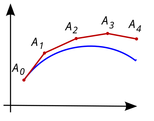
We consider a particle which at time \(t\) is at the position \(\vec{x}(t) = (x, y)\) and feels a velocity field \(\vec{u}(x, y, t)=(u, v)\). The position of the particle after a (very short) time difference \(\Delta t\) is approximately

\[\vec{x}(t+\Delta t) = \vec{x} + \vec{u}(x, y, t)\cdot\Delta t\]

where we neglected terms proportional to \(\Delta t^2\).

The subsequent locations of the particle at time \(t+2\Delta t\), \(t+3\Delta t\), … can then be found by moving the particle with the velocity field evaluated at the new position and at the new time.

The method of iteratively approximating a continuous differential equation only to this leading order in the independent variable (\(t\)) is often called the Euler Method.

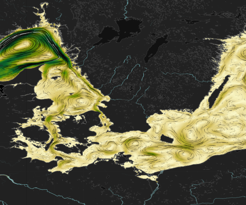
The flow field

We use a field of horizontal velocities at 5m depth from the Baltic Sea Physics Analysis and Forecast dataset distributed by the Copernicus Marine Service. The field comes as an Xarray dataset with dimensions for the horizontal position and time and with two variables containing the zonal component \(u\) and the meridional component \(v\) of the flow field \(\vec{u}(x, y, t)=(u, v)\).

While it is in principle possible to solve this project without ever explicitly downloading any data, by directly loading an Xarray dataset remote, the solution would be very slow. So there is file with the data we’re about to use:

"/home/jovyan/shared_materials/projects_data/01_baltic_sea_particle_drift_flow.nc"

To learn more about how this file was created, have a look at 01a_baltic_sea_particle_drift_preparation.ipynb.

Tasks

Solving the project can be broken down into multiple tasks:

1. In the formulation above, \(\vec{x}\) is usually thought of in units of meters and \(\vec{u}\) is usually in meters per second. But our problem lives on the curved surface of the Earth where positions are usually given in degrees longitude and degrees latitude. How do we adapt the equations for this?

2. Given an Xarray dataset with variables "u" and "v" on a grid of "longitude" and "latitude" values and with a "time" dimension, how to we find the velocity \(\vec{u}(x, y, t)\) from this dataset?

3. With \(\vec{u}\) at \((x, y, t)\) extracted from the Xarray dataset, how do we calculate (in code) the \((x, y, t)\) of the next position? And, supposing we want to visualize the whole track of the particle over time, how do we record the locations for multiple time steps?

4. How do you decide how big \(\Delta t\) should be?

5. Look at the flow field and find an interesting location and time to start a particle.

6. After recording the locations of the particle at multiple times \(t=t_0, t_0 + \Delta t, ...\), how do we store them for later use?

7. How can we visualize the particle trajectory in the context of the flow field?